Machine Learning SOC Estimation on a BMU, Verified Against a Twin

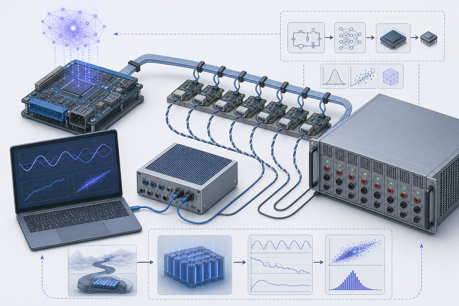
A recurrent SOC estimator that scores 1 % RMSE on held-out drive cycles can still show a 6 % error at 10 % SOC and −10 °C once it is wired into a real battery management unit. The network has not broken. It is operating where its training data was thin: the flat part of the LFP or NMC OCV curve, at a temperature it rarely saw, with inputs that arrive with a timing skew the offline dataset never had. Machine learning SOC estimation is easy to make look good and hard to bound. This piece covers the modelling side: how data-driven and hybrid estimators are structured so they fit a BMU-class microcontroller, and how a digital twin running in an emulator or HIL bench gives you the ground truth needed to measure error and drift instead of guessing at them.

Where machine learning SOC estimation sits in a high-voltage BMU

In a typical 400 V or 800 V pack, the BMU is the master. Cell-monitoring ICs on slave boards measure 12 to 18 cells each and pass data up an isolated daisy chain. Infineon's isoUART-based BMU reference designs are one example of this topology, and transformer- or capacitor-coupled SPI chains from other vendors follow the same pattern. The BMU reads pack current from a shunt or Hall sensor, collects cell voltages and a handful of temperatures, and runs the estimators.

Three properties of that architecture shape the estimator design more than the choice of network does.

Cell voltages arrive in bursts. A full chain readout typically takes somewhere between 10 ms and 100 ms. Current is sampled much faster, and an ECM-based observer expects voltage and current to be time-aligned. A 20 ms skew during a 300 A regen pulse, on a cell with 1 mΩ ohmic resistance, produces voltage-current pairs that do not belong together, with errors of tens of millivolts in the worst samples. A model trained on perfectly aligned lab data has never seen that.

Temperature is sparse. You might have one NTC per four to eight cells. The estimator works with an interpolated temperature field, not the cell core temperature.

The MCU is shared. Safety functions such as overvoltage, undervoltage, overcurrent and contactor control run on lockstep cores under ISO 26262. Estimation usually runs on a non-lockstep core or in a lower-ASIL partition, and it has to fit within a fixed time slice alongside balancing, diagnostics and communication.

Three ways to structure an ML-based estimator

I see three structures in practice. They differ mainly in what fails when the data runs out.

Structure	What the ML does	Typical size	Failure mode outside training range	Explainable to a safety assessor
Pure data-driven	Maps a history of V, I, T directly to SOC (MLP, GRU, LSTM, TCN)	5k–50k parameters	Silent, confident errors	Poorly
Hybrid residual	Corrects ECM terms (OCV offset, R0, RC parameters) inside an EKF/UKF	0.5k–5k parameters	Bounded by the clamp on the correction	Reasonably
ML parameter scheduler	Predicts ECM parameters from operating point and age features; the filter is unchanged	1k–10k parameters	Degrades to a mis-parameterised ECM	Well

My preference for production is the hybrid residual. A two-RC ECM with hysteresis, running inside an extended Kalman filter, captures most of the dynamics. Its known weaknesses are OCV hysteresis on LFP, temperature-dependent diffusion, and parameter drift with age, and those are exactly where a small learned correction pays off. Because the network only nudges a physical model, you can clamp its output to a physically plausible range. A failed network then shows up as a degraded ECM, not as a free-running SOC number.

/* Hybrid OCV: calibrated table plus a small int8 MLP residual, clamped */
float ocv_hybrid(float soc, float temp_c, float soh)
{
    float base = lut2d_interp(&ocv_lut, soc, temp_c);
    float r    = mlp_residual_q8(soc, temp_c, soh);  /* output in volts */
    if (r >  OCV_RES_MAX) r =  OCV_RES_MAX;          /* e.g. 0.015 V */
    if (r < -OCV_RES_MAX) r = -OCV_RES_MAX;
    return base + r;
}

Pure data-driven estimators also need a hard constraint. The simplest one is a charge-conservation bound: between two steps, the SOC estimate cannot move more than the coulomb count allows, plus a margin for the correction:

\left|\hat{z}_k - \hat{z}_{k-1}\right| \le \frac{|i_k|\,\Delta t}{3600\,Q} + \epsilon

Here $Q$ is capacity in Ah, $i_k$ is current in A, $\Delta t$ is the step in seconds, and $\epsilon$ is typically 0.1 % to 0.5 % per step. Any violation is logged as a diagnostic. In my experience this one line catches more field anomalies than any accuracy metric.

Fitting the estimator into a BMU microcontroller

The arithmetic is less frightening than people expect. Memory and worst-case execution time are the actual limits.

Consider a GRU with 32 hidden units and 4 inputs per cell (voltage, current, temperature, previous SOC). One step costs about $3 \times 32 \times (32 + 4) \approx 3.5\,\text{k}$ MACs. For 192 cells at 10 Hz, that is roughly 6.6 M MAC/s, which is comfortable on a 300 MHz automotive core even in floating point. The hidden state is the larger issue: 192 cells × 32 units × 4 bytes is about 24.6 kB of RAM that must persist and be protected. An LSTM doubles this because it also carries a cell state. The weights are small either way: around 3.5 k parameters fit in 3.5 kB of flash at int8.

Three decisions make the design fit:

Run the expensive model on representative cells only. Apply the full estimator to the minimum-voltage, maximum-voltage and one median cell. Run the ECM with a cheap correction on all cells. Pack SOC limits are set by the weakest and strongest cells anyway.
Quantise deliberately. Int8 weights with int16 or int32 accumulators are usually fine for MLP residuals. Recurrent states drift under aggressive quantisation over long horizons, so keep the hidden state in int16 or float.
Fix the worst-case execution time. Avoid data-dependent loop counts and dynamic allocation. Unroll the GRU into a fixed instruction sequence and measure it on target with caches cold.

The input skew described earlier should be handled in the model, not ignored. Either resample current to the timestamp of each cell's voltage, or train with injected skew so the network learns to tolerate it. The first option is cheaper and easier to defend.

AI state of health estimation runs on a different clock

SOH moves over weeks, not seconds. That changes the design completely. AI state of health estimation rarely needs to run in the inner loop. The BMU's job is to extract features reliably: capacity from partial charge segments between two rested OCV points, incremental-capacity (dQ/dV) peak positions during slow charging, and R0 from current steps with sharp edges. A larger model, on board or in the cloud, turns those features into capacity and resistance fade estimates. The updated SOH then feeds back into the SOC filter as $Q$ and as an input to the residual network.

The weak point is training data. Real aging trajectories under realistic duty cycles are expensive. Many published models are trained on constant-current cycling of small cylindrical cells, which tells you little about a prismatic cell in a pack that spends most of its life at 60 % SOC and 25 °C.

How does a BMS digital twin differ from the estimator's own model?

This distinction matters most for validation, and teams get it wrong regularly. The estimator contains a model. The digital twin is a separate, higher-fidelity model whose internal states, true SOC included, are known exactly at every step. It is the reference, not a copy of the estimator.

If you validate a hybrid ECM-EKF estimator against a twin built from the same two-RC ECM with the same parameters, you will see near-zero error and learn nothing. In inverse-problem terms, that is solving the problem with the model that generated the data. A useful BMS digital twin differs from the estimator's internal model in structure, in parameters, or in both. Good choices include:

a single-particle model with electrolyte (SPMe) or a full pseudo-two-dimensional (P2D) electrochemical model, parameterised for the cell chemistry;
a three-RC ECM with hysteresis and a coupled lumped thermal model, identified from a different test campaign than the one used to tune the estimator;
per-cell parameter spreads, for example ±3 % capacity and ±10 % R0 with a realistic distribution, so the twin represents a pack and not one idealised cell.

The twin runs faster than real time on a PC for software-in-the-loop work. Exported to a real-time target, it drives a cell emulator or HIL bench so the actual BMU hardware, with its ADCs, daisy chain and timing, sees the stimulus.

Quantifying estimator error and drift against the twin

With true SOC available at every sample, the error trace $e_k = \hat{z}_k - z_k$ becomes the main result. A single RMSE figure hides the cases that matter, so I report error by region and by mechanism. A minimum test matrix looks like this:

Convergence: start the estimator 20–30 % SOC away from truth and record the time to reach and stay within ±2 %.
SOC-band accuracy: maximum and 95th-percentile error in 10 % SOC bands, with the flat OCV region reported separately.
Temperature sweep: repeat the drive cycles at −20, 0, 25 and 45 °C, including temperatures between the training points.
Sensor faults: apply current offset and gain error, then measure the drift rate.
Unannounced aging: age the twin by 10–20 % capacity loss without telling the estimator, and record how long the SOH loop takes to catch up and what the SOC error is in the meantime.
Long-horizon drift: run 8–24 h of mixed cycling with no rest periods, so OCV recalibration cannot rescue the estimator.

Item 4 is where pure coulomb counting and weakly observable estimators fail. A current offset $I_\text{off}$ accumulates as:

\Delta z = \frac{I_\text{off}\, t}{3600\,Q}

A 50 mA offset over 8 h on a 100 Ah cell gives 0.4 %. That looks harmless until you note that a 500 mA offset, which a drifting Hall sensor can easily produce, gives 4 %. A well-designed hybrid estimator should hold the error bounded because the voltage measurement corrects it. A pure network trained on clean current data often will not.

The twin also supports embedded battery model validation in the narrow sense: checking that the on-target implementation matches the reference implementation. Run the same twin-generated stimulus through the float model on the host and the int8 model on the BMU, then compare outputs sample by sample. Quantisation error should be small, stationary and uncorrelated with SOC. Error that grows with time points to state accumulation in a recurrent layer. Error that correlates with SOC usually means the input scaling saturates at the ends of the range.

What the twin cannot tell you

A twin is only as good as its parameterisation. If the electrochemical model underestimates diffusion limits at low temperature, the estimator will look better on the bench than it will be in the vehicle. Close the loop with real-cell data at a few anchor points: at least one cold-temperature drive cycle and one aged cell measured on a cycler. Use those results to check that the twin's error predictions line up with real-cell error. Once they agree at the anchors, the twin is good enough to interpolate between them.

Frequently asked questions

Is machine learning SOC estimation more accurate than an EKF? Inside its training distribution, often yes, by a fraction of a percent. Outside it, a pure network can be much worse and gives no sign of it. Hybrid ECM-plus-ML estimators usually give the best worst-case behaviour.

Can an LSTM run on an automotive BMU microcontroller? Yes, if you size it per representative cell rather than per cell, keep the hidden units at 64 or fewer, and budget RAM for persistent states. Worst-case execution time and memory protection are the harder constraints, not MAC throughput.

Why not validate the estimator against coulomb counting from the cycler? Lab coulomb counting is a good reference for single cells, but it cannot give you per-cell truth in a pack, controlled parameter spread, or deliberate model mismatch. A digital twin can, and it can drive the actual BMU hardware.